Slice Analysis Panel and Measurements

The Slice Analysis panel lets you compute a range of measurements for each slice within an image stack or region of interest and then plot the selected measurements across all slices of the dataset. In addition, multiple panels can be opened to compare results from different views of your data or from multiple datasets.

To open the Slice Analysis panel, right-click the required view of your dataset or region of interest and then choose Start Slice Analysis in the pop-up menu. The objects analyzed in the panels shown below are an image (left) and a region of interest (right).

Slice Analysis panels

The option to analyze slices is also available in the Bone Analysis wizard (see Computing Slice-by-Slice Measurements).

You can do the following in the Slice Analysis panel:

Select the required measurements to analyze your data and plot the selected measurements across all slices.
Use masks and inverted masks to limit computations contained within a specific region.
Open multiple panels to compare results from different views of your data or from multiple datasets.
Export your results to a CSV file for further processing.

You can generate your own parameters for slice analysis with the Generic Slice Analysis Measurement Generator.

Per Slice Measurements for Images

The available per slice measurements for images are described in the table below.

Per slice measurements for images
Measurement	Description
Max	Is the maximum value extracted from the current image slice, as well as the corresponding minimum and maximum values that were extracted from the dataset as whole.
Min	Is the minimum value extracted from the current image slice, as well as the corresponding minimum and maximum values that were extracted from the dataset as whole.
Range	Is the data range extracted from the current image slice (maximum value minus the minimum value), as well as the corresponding minimum and maximum values that were extracted from the dataset as whole.
Mean	Is the mean data value extracted from the current image slice, as well as the corresponding minimum and maximum values that were extracted from the dataset as whole.
Median	Is the median data value extracted from the current image slice, as well as the corresponding minimum and maximum values that were extracted from the dataset as whole.
STD	Is the standard deviation extracted from the current image slice, as well as the corresponding minimum and maximum values that were extracted from the dataset as whole.
VAR	Is the variance extracted from the current image slice, as well as the corresponding minimum and maximum values that were extracted from the dataset as whole.

Per Slice Measurements for ROIs

The available per slice measurements for regions of interest are described in the table below.

Per slice measurements for ROIs
Measurement	Description
Voxel Count	The total number of voxels contained in the selected region of interest.
Moments of inertia	The moments of inertia listed below can be extracted from selected regions of interest: I_xx… The moment of inertia around the X axis, which is a measure of how material is distributed about the axis through the area centroid of each slice. Area moments of inertia are also known as second moments of area and characterize resistance to bending around a given axis. I_yy… The moment of inertia around the Y axis, which is a measure of how material is distributed about the axis through the area centroid of each slice. Area moments of inertia are also known as second moments of area and characterize resistance to bending around a given axis. I_max… The maximum moment of inertia, which is a measure of how material is distributed about the major centroidal axis, which is orthogonal to the minor centroidal axis. The maximum moment of inertia correlates to the maximum bending strength of a bone. Area moments of inertia are also known as second moments of area and characterize resistance to bending around a given axis. I_min… The minimum moment of inertia, which is a measure of how material is distributed about the minor centroidal axis, which is orthogonal to the major centroidal axis. The minimum moment of inertia correlates to the minimum bending strength of a bone. Area moments of inertia are also known as second moments of area and characterize resistance to bending around a given axis. J… The polar moment of inertia, which is the sum of any two perpendicular area moments of inertia (I_max + I_min) and characterizes resistance to torsion.
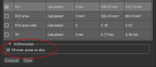
Pm (perimeter)	The total perimeter of the labeled voxels contained in the selected region of interest. Measurements of the periosteal perimeter can be extracted from cortical area segmentations, while measurements of the endocortical perimeter can be extracted from trabecular area segmentations. Note For perimeter calculations, you can choose to fill the inner areas of the region of interest on the image slices by checking the Fill inner areas on slice option. This will exclude the interior perimeter of closed areas within the ROI from the calculation.
ROI Area	The total area of the labeled voxels contained in the selected region of interest.
ROI area ratio	Computed as the number of voxels in the selected region of interest divided by the number of voxels in the slice. Note If a mask is applied, then the number of voxel in the ROI is the intersection of the mask and the selected ROI.
Th (mean thickness)	The mean thickness computed from the labeled voxels contained in the selected region of interest. Note For Bone Analysis computations, these measurements are usually extracted separately from cortical and trabecular bone segmentations.

Plot Tools

The tools at the top of the Slice Analysis panel let you save an image of the plot, change the default labels and formatting of the plot, as well as export the plotted values in the CSV file format.

Plotting tools
Item	Icon	Description
Save		Saves the figure as a bitmap image, vector graphic, or in the PDF file format. The figure can also be saved as raw data or PGF code. *Standard image files (.jpeg, .jpg, .png, .tif, .tiff extensions)… Saves the histogram or profile as a bitmap image in the screen resolution. Encapsulated postscript files (.eps extensions)…* Saves the histogram or profile as an encapsulated postscript or postscript file. These types of files have a selectable resolution and provide high-quality graphics for publications. PGF code for LaTeX (.pgf extension)… Saves the histogram or profile in the Portable Graphics file format. The standard LaTeX picture environment can be used as a front end for PGF merely by using the `pgfpict2e` package. Requires the XeLaTeX compiler. *Portable document format (.pdf extension)… Saves the histogram or profile in the Adobe PDF file format. Raw RGBA bitmap (.raw, .rgba extensions)… Saves the histogram or profile as a raw bitmap image file, in which the file contains only a list of pixel colors and nothing else. Scalable vector graphics (.svg, .svgz extensions)… Saves the histogram or profile in an XML-based vector image format. The SVG specification is an open standard developed by the World Wide Web Consortium (W3C). SVG images and their behaviors are defined in XML text files. WebP image format (.webp extension)…* WebP is a raster graphics file format developed by Google intended as a replacement for JPEG, PNG, and GIF file formats.
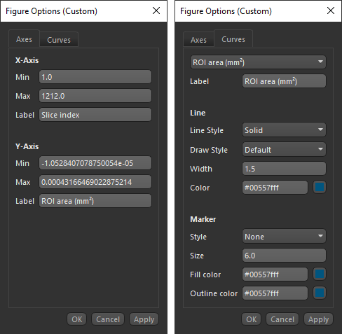
Settings		Opens the Figure Options dialog, shown below, in which you can select the plotted ranges, rename the labels of the axes, and choose a line style. Axes tab… Lets you edit the Min and Max values for each axis, as well as rename the label of each axis. Curves tab… Lets you choose a line style for the plot. Settings include the type of line applied, its width and color, and added marker.
Export to CSV		Exports the plotted values in the comma-separated values (.csv extension) file format. The delimiter for exporting in the CSV file format — comma, semicolon, or tab — can be selected in the Preferences dialog (see Miscellaneous Preferences). Note* All values related to regions of interest, such as the computed moments of inertia, perimeter, area, and thickness values, will exported in meters.